[kofi]
[paypal-donation]
Theoretical Background
Buckling analysis assesses the stability characteristics dictating the integrity limit of a structure.
Let us start with a linear equation of motion for a preloaded structure:
![]()
where M,C, K and Kd are mass, viscous damping, material and differential stiffness matrices (a matrix that is necessary to account for the change in potential energy associated with rotation of continuum elements under load; stiffness effects that depend linearly on displacements), and P(t) is a forcing function in time domain. To solve the equation shown above assume a harmonic solution of the form:
{u} = {Φ} sinωt
{Φ} the eigenvector or mode shape
ω is the circular natural frequency
The harmonic form of the solution means that all the degrees-of-freedom of the vibrating structure move in a synchronous manner. The structural configuration does not change its basic shape during motion; only its amplitude changes. If differentiation of the assumed harmonic solution is performed and substituted into the equation of motion, the following is obtained:
– ω 2[M] {Φ} sinωt + [K] { Φ} sinωt = 0
which after simplifying becomes
([K] – ω2[M]) {Φ} =0 (1)
This equation is called the eigenequation, which is a set of homogeneous algebraic equations for the components of the eigenvector and forms the basis for the eigenvalue problem. An eigenvalue problem is a specific equation form that has many applications in linear matrix algebra. The basic form of an eigenvalue problem is:
[A – λI] x = 0
where:
A = square matrix
λ=eigenvalues
I = identity matrix
x = eigenvector
In structural analysis, the representations of stiffness and mass in the eigenequation result in the physical representations of natural frequencies and mode shapes. Therefore, the eigenequation is written in terms of K, ω , and M as shown in Eq. (1) with ω2 = λ.
There are two possible solution forms for Eq (1):
1) If Det([K] – ω2[M]) ≠ 0 , the only possible solution is
{Φ} = O
This is the trivial solution, which does not provide any valuable information from a physical point of view, since it represents the case of no motion.
2) If Det([K] – ω2[M]) = 0, then a non-trivial solution ({Φ} ≠0) is obtained for
([K] – ω2[M]) {Φ} = 0
From a structural engineering point of view, the general mathematical eigenvalue problem
reduces to one of solving the equation of the form:
Det([K] – ω2[M])
or
Det([K] – λ [M])
with λ = ω2
The determinant is zero only at a set of discrete eigenvalues λi. There is an eigenvector {Φi} which satisfies and corresponds to each eigenvalue. Therefore, can be rewritten as:
[K – ωi2M] {Φi} = 0 i = 1,2,3,4,…
Each eigenvalue and eigenvector define a free vibration mode of the structure. The i-th eigenvalue λi is related to the i-th natural frequency as follows:
fi = ωi/2π
where:
fi = i-th natural frequency
ωi = √ λi
The number of possible eigenvalues and eigenvectors is equal to the number of degrees-of-freedom that have mass or the number of dynamic degrees-of-freedom. When a linear elastic structure is vibrating in free or forced vibration, its deflected shape at any given time is a linear combination of all of its normal modes:
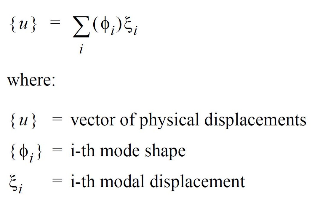
Returning to the Eq. (1), the differential stiffness has to consider and it is created by the initial stress due to preloads, and it may include the follower stiffness if applicable. Ignoring the damping term to avoid complex arithmetic, an eigenvalue problem may be formulated as:
![]()
which is a governing equation for normal mode analysis with a preload, but it could be recast for a dynamic buckling analysis at a constant frequency.
For a static buckling, the inertia term drops out because the frequency of vibration is zero:
![]()
in which {Φ} represents virtual displacements. A non-trivial solution exists for an eigenvalue that makes the determinant of [K + Kd] vanish, which leads to an eigenvalue problem:
![]()
where λ is an eigenvalue which is a multiplier to the applied load to attain a critical buckling load. If there exists static preloads other than the buckling load in question, the above equation should include additional differential stiffness:
![]()
in which differential stiffnesses are distinguished for constant preload and variable buckling load. The buckling analysis with an excessive preload can render wrong solutions.
The analysis is restricted to linear elastic material and infinitesimal deformations. The static load P is applied in the first subcase. This eigenvalue problem is solved in the second subcase. Kd is the differential stiffness which is a function of stress due to the static load P from the first subcase. The problem is solved for the eigenvalues λi and eigenvectors Φi. The critical buckling loads are Pi-crit= λi *P.
How to perform a linear Buckling in Nastran
When the FEM has several load cases, before to perform buckling analysis by Nastran, it is necessary to understand which load cases are critical for the structure. It could be determine by detecting the load cases with high compressive loading. In general the selection criteria is the Minimum Principal Stress (take in to account the most negative value, since the negative concerns the compression), max/min shear stress, and the maximum compression stress in x or y direction (x and y in the plane of the cquad element). In particular for the composite materials could be enough the Minimum Principal Stress. Once you detected the critical load cases (for example 8 loads most critical), you have to setup your Nastran file putting the key work highlighted in yellow in the following figure (click on).
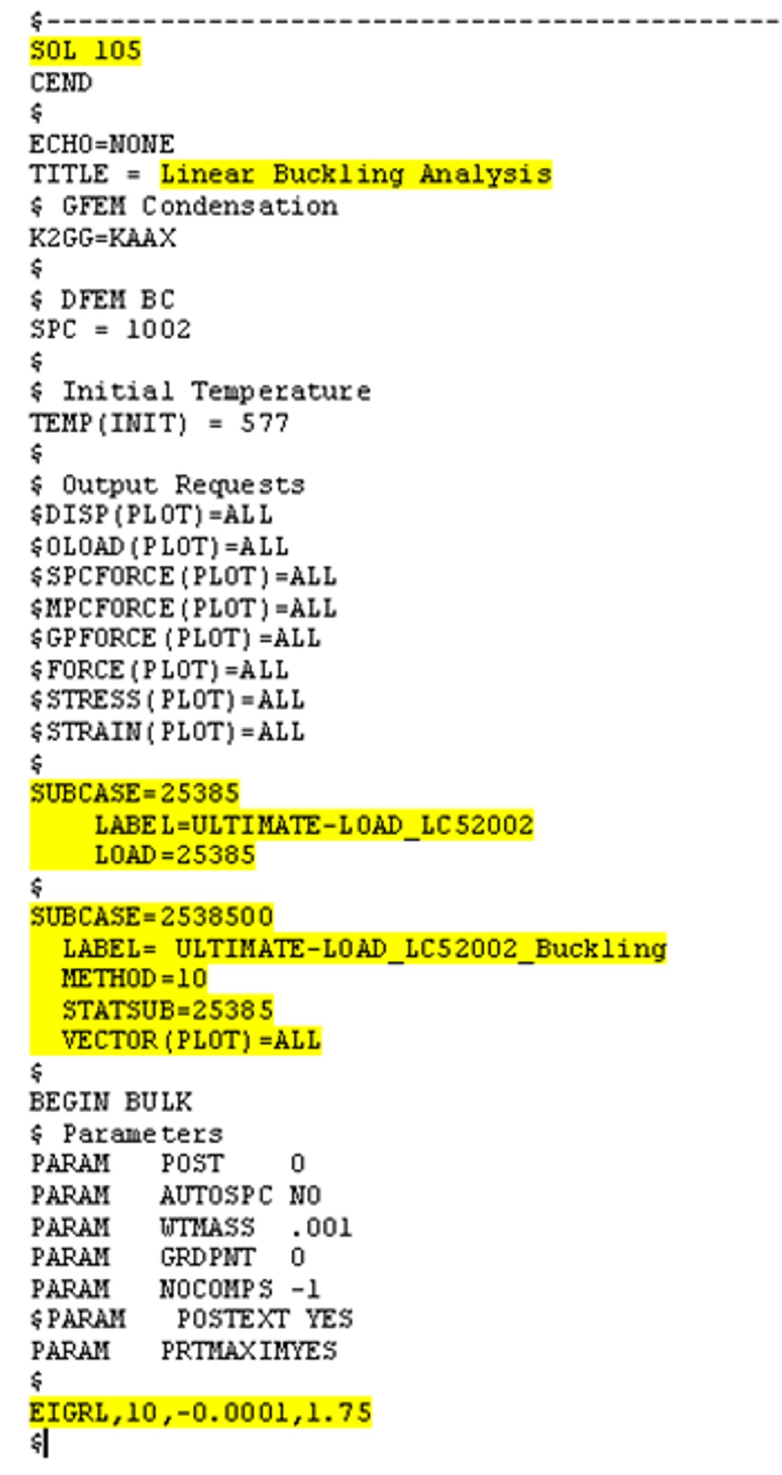
For each critical load case you have to perfor the Buckling analysis. In this example the critical one is the load case named “25385”. The numerical solution for the linear Buckling is “SOL 105”. The “SUBCASE=2538500” is linked to “SUBCASE=25385” (by STATSUB), and it is linked to EIGRL by “METHOD=10”. By EIGRL you can set the analysis performing, in this case the results will consider all the eigenvalues between -0.0001 and 1.75. The results can be read in the f06 file got after the running (see below, click on).

Obviusly the minimum (positive) eigenvalue has to be at least greater then 1.00 (but usually it is knocked down by a safe factor, thus usually the eigenvalue has to be greater 1.30). In the results below are shown for each eigenvalue the properly frequency (“RADIANS” for second, and “CYCLES” for second) and the “GENERALIZED MASS” and “GENERALIZED STIFFNESS” (see below the Rayleigh’s equation for a linear elastic structure)

The third and fifth Eq. shown in the figure above are known as as the orthogonality property of normal modes, which ensures that each normal mode is distinct from all others. Physically, orthogonality of modes means that each mode shape is unique and one mode shape cannot be obtained through a linear combination of any other mode shapes. In addition, a natural mode of the structure can be represented by using its generalized mass and generalized stiffness. This is very useful in formulating equivalent dynamic models and in component mode synthesis, thus the numerical calculation is easier.
Meshing hints
The mesh density must to be adequate in order to capture the highest number of semi-waves. If you use shell elements, for example in case of buckling due to compression, at least N ≥5 per semi-wave is recommended for the mesh density, instead for the buckling due to the shear, is recommended N≥10. The elements have to be oriented all with same element sys orientation, in order to consider correctly the contribution of all elements.
Errors
When you have a FE model with offset you can get an error like this:
*** USER FATAL MESSAGE 6174 (EBARD)
BAR ELEMENT (EID=159) WITH OFFSETS REQUIRES MDLPRM,OFFDEF, VALUE TO BE SPECIFIED,
PLEASE REFER TO THE QUICK REFERENCE GUIDE FOR DOCUMENTATION ON MDLPRM,OFFDEF.
In this case you need to use the MDLPRM parameter to avoid this inconvenient. It is recommended the following setting: MDLPRM,OFFDEF,LROFF. In this manner you will take into account of the differential stiffness due to the offset. Note, this parameter is usable only from Nastran 2012, not by previous versions.
[kofi]
[paypal-donation]