1 – Introduction
2 – Aerodinamic for compressible gas – Basic principles
4 – Turbogas cycle
5 – Turbofan
5.1 Turbofan with separated flows
5.2 Turbofan with associated flows
6 – Combustion chamber
7 – Inlet
8 – Nozzle
9 – Turbine Engine
2.1 Ideal Gas Law
For the study of the engines are frequently used the ideal gas with constant properties as approssimation, and assumes that the conditions of the flow within ducts vary only along the direction of the axis of the duct himself, taking the equations that describe the motion of a compressible flow in case of flow almost unidimensional.
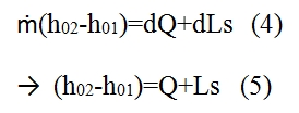
The behaviour of ideal gas is described by the equation of state:
p=ρRT.
Where R is a gas constant. R= R/M, where R is an universal gas constant, M is the molecolar weight; for air M = 29 Kg/kmol and R= 8314JK-1Kmol-1. Ρ is the density and it is equal to m/V.
To have an idea of the usefulness of this equation in the following figures is shown the trend of Z factor (Z = p/ ρRT, that is equal to 1 for an ideal gas) for H2O and CO2 (typical gases producted after the combustion). As is noticable Z is really close to 1 at tipical temperatures and pressures present in combustion chamber. The charts are is function of the reduced temperature Tr and reduced pressures Pr, with Tr= T/Tcr and Pr =P/Pcr, where the subscript „cr“ is referred to maximum value that identify the equilibrium condition with liquid and vapour state coesistence.

Fig 3 – Z for H2O(Tcr=647.3 K, pcr=22.12 MPa).
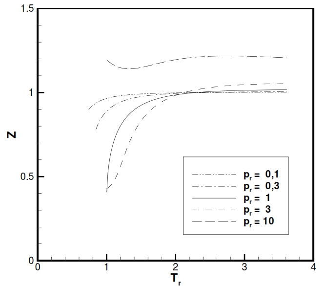
Fig 4 – Z for CO2 (Tcr=304.4 K, pcr=7.38 MPa).
Instead the parameter Cp (specific heat at constant temperature) and ϒ = Cp / Cv (Heat capacity ratio) for the gases used as propeller with high temepratures, doesn´t show properly an ideal behaviour as is highlighted in the following figures. Nevertheless for the our study we make the hypothesis of ideal behaviour for Cp and ϒ, and for a better description it is possible to use some equation for Cp versus temperaure like Cp = -2.23488 · 1010T-3+3.09372 · 108T-2-1.52622 · 107T-1.5+1335.1+1.45566 · 10-4T1.5.

Fig 5 – Chart_CP_T
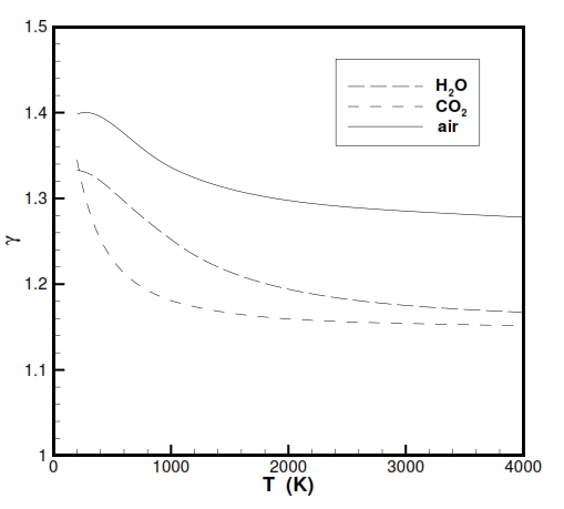
fig 6 – Chart_Gamma_T
2.2 Speed of sound
For an ideal gas, the speed of sound a, is calculated considering the gas properties and the temperature. Thus a can be expressed as state variable:
![]()
where ϒ = Cp / Cv, R is the gas constant, T is the temperature.
2.3 State Parameters at stagnation condition
We define as conditions of stagnation, the conditions that the fluid assumes when is decelerated till to zero velocity. For the deceleration process can be assumed :
- Adiabatic without work exchange; under these hypothesis we can define h0, e0, T0, a0.
- Adiabatic, isentropic and without work exchange; under these hypothesis we can define P0, ρ0.
The relationships between the parameters at stagnation point, static parameters and Mach number are:
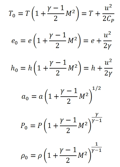
Where e0 is the internal energy. The enthaphy and the internal energy can be expressed with respect a reference temperature Tref , for example by this formula h=href+Cp(T-Tref), with href =CpTref .
2.4 Quasi-unidimensional stationary flow
By the hypothesis of quasi-unidimensional flow the study is simplier in case of variation of area within ducts, friction or heat exchange.
The hypothesis of quasi-unidimensional flow implies:
- Constant properties of each cross section of the duct (normal to the axis);
- Properties depend on a single spatial variable (the abscissa along the axis of the duct).
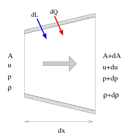
Fig 7- Control volume to study the quasi-unidimensional stationary flow
These hypothesis are sufficient for average values of the flux. In the following paragraphs are considered the equation for conservation of mass, the quantities momentum equation, the energy equation in differential form by using the scheme in fig 7 and considering with positive sign the work and heat absorbed by the fluid.
Conservation of mass
With stationary conditions the mass of gas contained within the control volume (Fig. 7) remains constant. The flow rate of the gas has to be equal in entrance and in outgoing:
ρuA=(ρ+dρ)(u+du)(A+dA)
sine the flow rate is constatnt we have:
d(ρuA)=0
Using the logaritmic form we have:
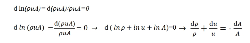
Where as second member is reported dA/a by means is possible to modify the parameters along the duct.
Quantities Momentum equation
The difference of input momentum and output momentum through the control volume, is equal to resultant of forces applied to the fluid.
![]()
The resultant of forces is equal to the sum of pressure forces acting externally on the control volume plus the friction forces:
![]()
Semplifing and neglecting the higher order infinitesimal we have:
![]()
Where
![]()
(P is the perimeter of the duct)
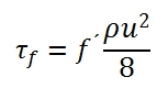
Dividing by ρAu2 we have:
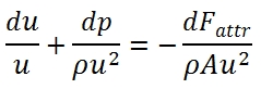
f´ is the friction factor, and it depeds of the Reynolds number, and roughness of the duct surfaces.
Conservation of energy
Considering the duct shown in Fig 8, the energy per unit mass that enter in the duct is equal to the sum of the specific internal energy e1 and the specific kinetic energy u12/2.
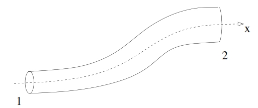
Fig 8 – Quasi-unidimensional duct
Since for each time unit enter in the duct the fluid mass equal to the flow ṁ and, due the stationary hypothesis, the conditions 1 and 2 are constant, the ṁ is constant along the duct, the variation of energy in the duct is equal to:
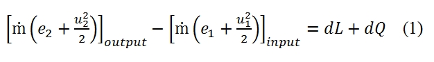
Therefore the difference between the input energy and output energy is equal to the work carried out on the fluid plus the heat provided to the fluid in the time unit. Denoting with dLs the work provided externally by a fan placed along the duct, and since the fluid velocity is nought on the walls therefore their work is null, we have:
![]()
where with piAiui is denoted the work of the pressure in the section 1 and 2. By substituting the equation 2 in 1, and since ṁ=ρ1A1u1= ρ2A2u2 we have:

Since the relationship between the entalpy and internal energy is given by h=e+p/ρ, and since the total entalpy is equal to h0=h+u2/2, we have:
The result is then that provide heat or carry out work on a flow causes a change of its total enthalpy which is then the energy content of the flow. Conversely a decrease in the total enthalpy indicates cooling of flow or work done by the fluid on a blading. The result obtained by (4) can be applied to the infinitesimal element shown in Fig 7. In (5) are shown the heat and work per mass and time unit. We will use the differential form of (5) neglecting the Ls since make no sense consider it in an infinitesimal volume, thus we have:
dh0=dQ
Equations for unidimensional flux
Equations of one-dimensional flow, equations of conservation of mass, quantities momentum and energy in differential form allow to write the system that determines the state of the flow:

The terms in the second member are known terms, and then determine the particular solution of flow. The flow in a certain section abscissa x is not known whether notes are two state variables and the velocity (or equivalently, the Mach number), therefore is convenient to rewrite the system in terms of three unknown variables, which It may be done by using the state equations.
The system can be rewrite as a function of Mach number M, dp / p, dM / dT and M / T. Adopting logarithmic derivation, we can obtain easily the following differential equations:
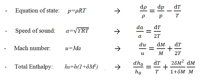
Where δ=(ϒ-1)/2. Therefore the system to solve is built up by these equations:
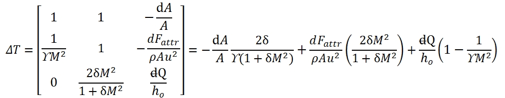
That it can be write in matrix form:
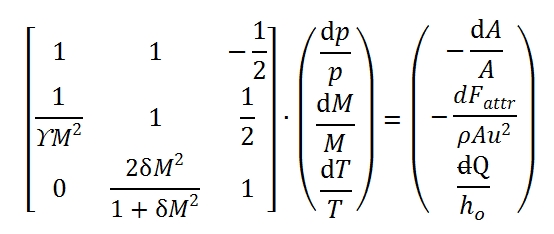
the solution can be expressed as a function of 3 × 3 determinants that can be easily calculated:
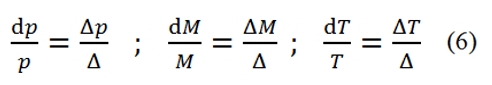
The Δ is the determinant of the matrix.
Calculating of determinants

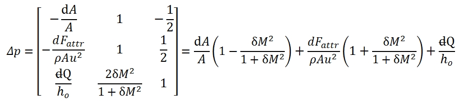
Δp is the determinant of the matrix that can be obtained from coefficient matrix by replacing the first column with the column of the known terms:
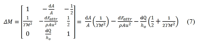
ΔM is the determinant of the matrix that can be obtained from coefficient matrix by replacing the second column with the column of the known terms:
ΔT is the determinant of the matrix that can be obtained from coefficient matrix by replacing the third column with the column of the known terms:
As result each of the unknowns can be expressed as the sum of three terms, each relating to the effect of one of the three source terms (variation of area, friction, heat flow). In general, the source term appears multiplied by a function of M. For own convenience the solution. It may be shown in a table (Tab. 1). In the table in addition to the variables that have been used to solve the system, are also reports the changes of total pressure and velocity, which can be expressed as a function of p, T, M and source terms. The total pressure is of particular interest as it is a measure of the flow capacity to do work and therefore the possibility of using it for propulsion (note that the total enthalpy It’s a measure of total energy of flow).
The determinants of the motion equations are equal to zero for M = 1. This condition identify the position of critical section. For instance, a flux with negligible friction (dFattr≈0), without any exchange of heat (dQ=0), from (7) in this case, the critical section id that one with dA=0, the section with minimum area of the duct.
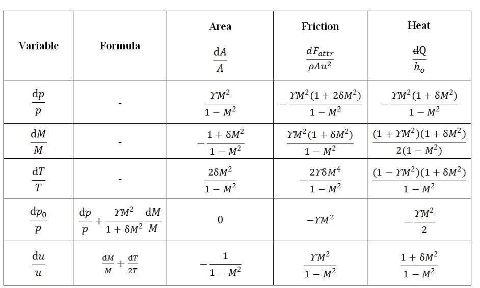
Tab 1: Coefficients of the general solution for quasi-unidimensional stationary flows
Integral Equations
The conservation equations can be written in finite form by intragration of the differential equations or extracting them directily. Of particular interest are the solutions obtained considering the effect of a single forcing term in the system of equations of motion, and therefore set aside the remaining two:
- Isentropic Flux: ṁ=ρuA=cost, T0=cost, p0=cost. By this hypothesis we can extract some simple formula that correlates the ratio between the section areas and Match number present in them, and consequently all the variables (see below the law´s Areas).
- Flux in duct with constant section with friction and without heat exchange (Fanno flux): T0=cost, ρu=cost. The development of the calculation of this flow is not reported here.
- Flux in duct with constant section without friction and with heat exchange (Rayleigh flux):
ρu=cost, p+ ρu2=cost. The development of the calculation of this flow is not reported here.
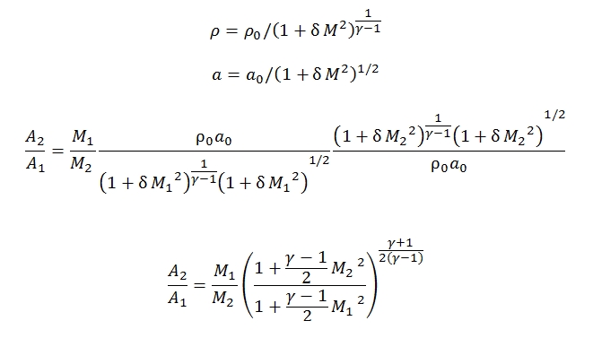
Law´s Areas for isentropic flow
In a flow without friction and without heat exchange entropy is constant, as it can easily derive the Gibbs´s formula:
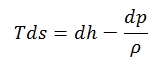
Where dh can be express as –udu, dp/p by the conservation energy and quantities momentum equations. By the equations explained above is easy to obtain a formula that correlates Match number and isentropic flux (no friction, no heat exchange, no work external exchange):
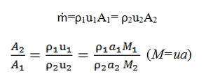
Since the state parameters with this hypothesis are constant we have:
Mass flow for isentropic condition with M=1
The mass flow can be expressed as a function of throat area At of the duct, and if the flow is critical we have:
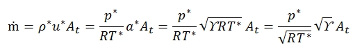
Since for M=1 we have:
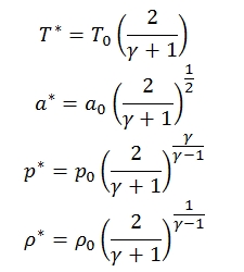
Therefore:
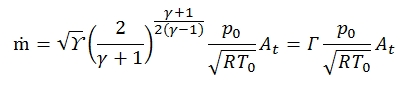
Where Γ is defined as:

It is graphically reported in figure below, tipocally Γ has values about 0.65 and 0.68. By the equation shown above we can deduct that for an isoentropic flux (T0=cost, p0=cost), fixed the stagnation condition and the throat area, the mass flow in critical condition (M=1) is fixed.

Fig 9: Γ versus γ
[smartslider3 slider=”2″]